Standalone Examples

This page is the figure gallery. For the fastest API overview, equations, and shape conventions, start with usage.md.

The maintained standalone entry points are:

• examples/standalone_quickstart.py for a one-file smoke test

• examples/standalone_gallery.py for the figure-producing workflows below

The first three examples here are direct excerpts from examples/standalone_gallery.py and require contimod_graphene plus matplotlib.

1. ABC Trilayer: Full Model vs 2-Band Reduction

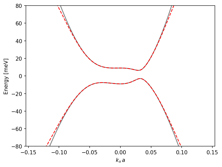
Physics: compare the full six-band rhombohedral trilayer Hamiltonian against the low-energy two-band reduction. The maintained example pins Delta=0.0 so the plot isolates the outer-layer bias U, rather than the preset’s small built-in Delta=-1.15 meV offset.

Near neutrality, the low-energy branch follows the expected ABC scaling $E \propto k^3$.

import numpy as np
import jax
import jax.numpy as jnp
import matplotlib.pyplot as plt
import contimod_graphene as cg

params = cg.GrapheneTBParameters.preset("tlg").replace(U=10.0, Delta=0.0)
model = cg.RhombohedralMultilayer(n_layers=3, params=params)

k_lin = 0.28 * jnp.linspace(-0.5, 0.5, 400)
ks = jnp.stack([k_lin, jnp.zeros_like(k_lin)], axis=-1)

Hs_full = model.hamiltonian_batch(ks)
bands_full = jnp.linalg.eigvalsh(Hs_full)  # shape (400, 6)

Hs_low = jax.vmap(
    lambda kx, ky: model.two_band_hamiltonian(kx, ky),
    in_axes=(0, 0),
)(*ks.T)
bands_low = jnp.linalg.eigvalsh(Hs_low)  # shape (400, 2)

mid = len(k_lin) // 2
print(np.round(np.asarray(bands_full[mid]), 3))
print(np.round(np.asarray(bands_low[mid]), 3))
print(np.round(float(bands_low[mid, 1] - bands_low[mid, 0]), 3))

fig, ax = plt.subplots()
for band in bands_full.T:
    ax.plot(k_lin, band, color="black", linewidth=1.5, alpha=0.5)
for band in bands_low.T:
    ax.plot(k_lin, band, color="red", linewidth=1.5, linestyle="--", alpha=0.9)

ax.set_xlabel(r"$k_x\,a$")
ax.set_ylabel("Energy [meV]")
ax.set_ylim(-80, 80)
plt.show()

[-382.508 -377.508   -9.014    9.014  377.508  382.508]
[-9.014  9.014]
18.028

Interpretation: at k=0, the 2 x 2 model reproduces the low-energy pair of the full six-band Hamiltonian, while the other four bands stay hundreds of meV away.

2. Bilayer Landau-Level Fan

Physics: diagonalize the dense LL-basis Hamiltonian $H_{\mathrm{LL}}(B)$ as a function of magnetic field and plot the eigenvalues as a fan diagram.

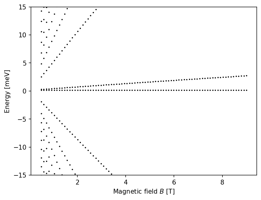
For n_layers=2, the Bernal and rhombohedral kernels describe the same AB bilayer connectivity. The maintained example keeps the public BernalMultilayer entry point for consistency with the rest of the docs.

import jax.numpy as jnp
import matplotlib.pyplot as plt
import numpy as np
import contimod_graphene as cg

params = cg.GrapheneTBParameters.preset("blg").replace(U=0.0)
model = cg.BernalMultilayer(n_layers=2, params=params)

B_values = jnp.linspace(0.5, 9.0, 80)

eigvals = []
for B in B_values:
    H = model.landau_level_hamiltonian(float(B), n_cut=40)
    eigvals.append(np.linalg.eigvalsh(np.asarray(H)))  # 158 levels for BLG at n_cut=40

sample = np.linalg.eigvalsh(
    np.asarray(model.landau_level_hamiltonian(10.0, n_cut=8, valley="K"))
)
closest = np.sort(sample[np.argsort(np.abs(sample))[:8]])
print(np.round(closest, 3))

fig, ax = plt.subplots()
for B, e in zip(np.asarray(B_values), eigvals):
    ax.plot(np.full_like(e, B), e, "k.", ms=2)

ax.set_xlabel(r"Magnetic field $B$ [T]")
ax.set_ylabel("Energy [meV]")
ax.set_ylim(-15, 15)
plt.show()

[-89.455 -66.373 -39.829   0.195   4.361  50.655  82.021 109.28 ]

Interpretation: this shows the near-zero bilayer levels and the first higher LL branches before you commit to the full fan plot.

3. ABA Trilayer Zero-Field Bands

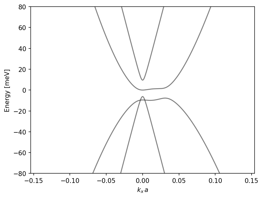
Physics: compute the zero-field six-band ABA trilayer dispersion along a one-dimensional $k_x$ scan.

This is intentionally a custom-parameter example. The package does not currently ship a dedicated ABA trilayer preset, so the cleanest maintained path here is GrapheneTBParameters.from_dict(...).

import numpy as np
import jax.numpy as jnp
import matplotlib.pyplot as plt
import contimod_graphene as cg

graphene_params_ABA = {
    "gamma0": 3100,
    "gamma1": 370,
    "gamma2": -19,
    "gamma3": 315,
    "gamma4": 140,
    "gamma5": 20,
    "U": 0.0,
    "Delta": 18.5,
    "delta": 3.8,
}

k_lin = 0.28 * jnp.linspace(-0.5, 0.5, 400)
ks = jnp.stack([k_lin, jnp.zeros_like(k_lin)], axis=-1)

params_aba = cg.GrapheneTBParameters.from_dict(graphene_params_ABA)
model_aba = cg.BernalMultilayer(n_layers=3, params=params_aba)

Hs = model_aba.hamiltonian_batch(ks)
bands = jnp.linalg.eigvalsh(Hs)  # shape (400, 6)

print(np.round(np.linalg.eigvalsh(np.asarray(model_aba.hamiltonian(0.0, 0.0))), 3))

fig, ax = plt.subplots()
for band in bands.T:
    ax.plot(k_lin, band, color="black", linewidth=1.5, alpha=0.5)

ax.set_xlabel(r"$k_x\,a$")
ax.set_ylabel("Energy [meV]")
ax.set_ylim(-80, 80)
plt.show()

[-514.476  -15.45    -9.25    -0.25    18.75   532.076]

Interpretation: the outer pair sits far from neutrality, while the inner four bands show the familiar ABA mix of monolayer-like and bilayer-like low-energy structure.

4. Quickstart And Notebooks

examples/standalone_quickstart.py is the smallest maintained script and writes a JSON summary of shapes, band extrema, and sample eigenvalues. It is the fastest way to check that the public API works on your machine.

contimod_example.ipynb is intentionally the one notebook in examples/ that assumes the separate downstream contimod package is installed.

The older notebooks bandstructure_plots.ipynb, bernal_bands_LL.ipynb, and landau_level_fans.ipynb remain useful exploratory references, but the maintained default workflow should start from examples/standalone_quickstart.py, examples/standalone_gallery.py, or the short snippets in usage.md.