Tutorial 3 — Haldane Model & Topology

Notebook: extra/tutorial/Tutorial3_Haldane.ipynb

Explore how to induce topological gaps in graphene-like systems and compute observables that diagnose Chern insulating phases.

Learning goals

Introduce complex next-nearest-neighbour hoppings via Operators.addhaldane!.
Study phase diagrams by sweeping Haldane mass and onsite potentials.
Evaluate Berry curvature and Chern numbers with Spectrum utilities.
Visualise chiral edge states on ribbon geometries.

Prerequisites

Outcomes from Tutorial 2 (band-structure workflows).
Optional: knowledge of topological band theory terminology.

Workflow outline

Model setup — Build a honeycomb lattice and baseline graphene Hamiltonian.
Haldane term — Apply Operators.addhaldane!(hops, lat, φ; spinhalf=true) and optionally stack with sublattice imbalance.
Parameter scans — Use simple loops or range objects to inspect phase transitions. Store observables with @save or by writing CSV/JSON.
Topological invariants — Invoke Spectrum.chern(hops, ks; ...) or related helpers to compute Chern numbers.
Ribbon perspective — Transform to ribbon geometries (see extra/examples/graphene/ribbon_haldane.jl) and plot edge-localised states.

Live example

figdir = joinpath(pwd(), "figures")
mkpath(figdir)
nothing

cherns = Spectrum.getcherns(hops, 15, 15)
println("Chern numbers (lowest two) = ", cherns[1:2])

Chern numbers (lowest two) = [0.9999999999999999, -1.0]

p = plot(
    getbands(hops, ks, [valley]);
    ylabel="ε/t",
    marker=:none,
    size=(420, 260),
    title="Haldane model band structure",
    colorbar=true,
    colorbar_title="valley"
)
savefig(p, joinpath(figdir, "haldane_bands.svg"))
nothing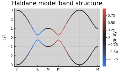

Berry curvature map

kgrid, berry = Spectrum.berry(hops, 20, 20, [1])
vals = filter(!isnan, abs.(berry[:]))
maxval = isempty(vals) ? 1.0 : Statistics.quantile(vals, 0.98)
p = scatter(
    (Structure.Lattices.getB(lat) * hcat(reshape(kgrid, :, 1)...))[1, :],
    (Structure.Lattices.getB(lat) * hcat(reshape(kgrid, :, 1)...))[2, :];
    marker_z = vec(berry),
    markerstrokewidth=0,
    markersize=3,
    colorbar=true,
    clims=(-maxval, maxval),
    markercolor=:RdBu,
    xlabel="k₁",
    ylabel="k₂",
    size=(360, 280),
    legend=false,
    aspect_ratio=:equal
)
savefig(p, joinpath(figdir, "haldane_berry.svg"))
nothing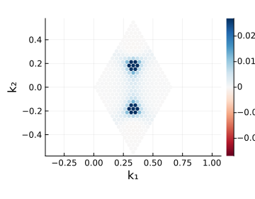

Phase diagram (coarse grid)

using LaTeXStrings
phi_vals = LinRange(-π, π, 25)
m_vals = LinRange(-1.2, 1.2, 25)
h0 = Operators.graphene(lat; mode=:nospin, format=:dense)
C = fill(0.0, length(phi_vals), length(m_vals))
for (i, ϕ) in enumerate(phi_vals), (j, Δ) in enumerate(m_vals)
    local_model = deepcopy(h0)
    Operators.addsublatticeimbalance!(local_model, lat, Δ)
    Operators.addhaldane!(local_model, lat, 0.2; ϕ=ϕ)
    C[i, j] = sum(Spectrum.berry(local_model, 10, 10, [1])[2])
end
p = heatmap(
    phi_vals ./ π,
    m_vals,
    transpose(round.(C; digits=2));
    xlabel=L"\phi/\pi",
    ylabel=L"m/t_2",
    colorbar_title="Chern",
    size=(420, 240),
    color=:seismic
)
savefig(p, joinpath(figdir, "haldane_phase.svg"))
nothing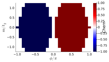

Ribbon dispersion

N = 20
lat_ribbon = Structure.Lattices.reduceto1D(Geometries.honeycomb(), [[1, 1] [N, -N]])
h_ribbon = Operators.graphene(lat_ribbon; mode=:nospin, format=:dense, cellrange=1)
Operators.addhaldane!(h_ribbon, lat_ribbon, 0.25)
position = Operators.positionalong(lat_ribbon, Structure.Lattices.basis(lat_ribbon, 2); rescale=true, center=true)
ks_ribbon = kpath(lat_ribbon; num_points=140)
bands_ribbon = getbands(h_ribbon, ks_ribbon, position)
p = plot(
    bands_ribbon, 1;
    ylabel="ε/t",
    colorbar_title="transverse position",
    csymmetric=true,
    markersize=1.5,
    size=(450, 260)
)
savefig(p, joinpath(figdir, "haldane_ribbon.svg"))
nothing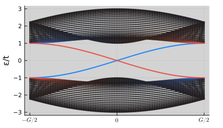

Nested Wilson Loops (SSH×SSH snapshot)

using LatticeQM.Structure.Lattices: Lattice, addbasis!, addorbital!, addextra!
function SSHxSSH(t1X, t2X, t1Y, t2Y)
    lat = Lattice()
    addbasis!(lat, [1, 0]); addbasis!(lat, [0, 1]); addextra!(lat, "sublattice")
    addorbital!(lat, [0,   0,   2]); addorbital!(lat, [1/2, 0,   4])
    addorbital!(lat, [0, 1/2,   3]); addorbital!(lat, [1/2, 1/2, 1])
    lat.specialpoints = LatticeQM.Geometries.kdict_sq
    h = DenseHops()
    h[[0,0]] = zeros(ComplexF64, 4, 4)
    h[[0,0]][3,1] = t1X; h[[0,0]][2,3] = -t1Y; h[[0,0]][4,2] = t1X; h[[0,0]][1,4] = t1Y
    h[[0,0]] += h[[0,0]]'
    h[[1,0]] = zeros(ComplexF64, 4, 4); h[[1,0]][3,1] = t2X; h[[1,0]][2,4] = t2X; h[[-1,0]] = h[[1,0]]'
    h[[0,1]] = zeros(ComplexF64, 4, 4); h[[0,1]][2,3] = -t2Y; h[[0,1]][4,1] = t2Y; h[[0,-1]] = h[[0,1]]'
    lat, h
end
latSSH, hSSH = SSHxSSH(0.5, 1.0, 0.5, 1.0)
pol1, U1, pol2, U2 = Spectrum.NestedWilson2D(hSSH, 60, 60, 1:2)
p = plot(scatter(collect(1:length(pol1[:,1])), pol1[:,1]; ms=3.0, label="1"),
         scatter(collect(1:length(pol1[:,2])), pol1[:,2]; ms=3.0, label="2");
         size=(420, 260), xlabel="k₂ index", ylabel="polarisation k₁")
savefig(p, joinpath(figdir, "sshxssh_wilson.svg"))
nothing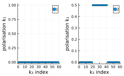

Validation checklist

Confirm Chern numbers match the expected ±1 quantisation when phases wrap.
Create plots of Berry curvature hotspots and verify symmetry.
Compare ribbon spectra with bulk band gaps for consistency.

Suggested extensions

Couple the model to linear-response routines in LinearResponse to compute Hall conductivities.
Introduce disorder or electric fields to study robustness of edge channels.
Export topological markers for later visualisation using scripts in extra/examples/.