Tutorial 1 — Structure & Geometry

Notebook: extra/tutorial/Tutorial1_Structure.ipynb

This tutorial introduces lattice construction in LatticeQM, from specifying primitive vectors manually to using the extensive catalogue under LatticeQM.Geometries. By the end you will be comfortable building lattices, inspecting their coordinates, and producing quick sanity plots.

Learning goals

• Understand how LatticeQM.Structure encodes lattice vectors and orbital positions.
• Instantiate standard geometries (square, honeycomb, multilayer stacks).
• Visualise sites and bonds for 2D systems and inspect neighbour shells.

Prerequisites

• Julia basics and familiarity with matrix/vector notation.
• Plots.jl installed (Pkg.add("Plots")) for quick visual checks.

Workflow outline

1. Manual lattices — Define primitive vectors and fractional coordinates, e.g. lat = Lattice([1 0; 0 1], [[0, 0] [0.5, 0.5]]).
2. Predefined geometries — Load helpers such as lat = Geometries.honeycomb() or Geometries.honeycomb_twisted(n).
3. Inspection utilities — Query Structure.coordinates(lat), Structure.getA(lat), or Structure.get_positions(lat) to confirm unit cell data.
4. Neighbour analysis — Use Structure.getneighbors(lat; cutoff=...) to tabulate bonds or export them to downstream calculations.
5. Plotting — Render a quick layout with plot(lat; repeat=[0:1,0:1]) to confirm angular orientation and stacking.

Note on coordinates: Structure.Lattices.coordinates(lat) returns fractional positions in units of lattice vectors. Use Structure.Lattices.positions(lat) to obtain Cartesian coordinates (A * coordinates).

Live example — manual construction

figdir = joinpath(pwd(), "figures")
mkpath(figdir)
nothing

println("Lattice vectors A =")
Structure.Lattices.getA(lat)

3×2 Matrix{Float64}:
  1.5       1.5
 -0.866025  0.866025
  0.0       0.0

println("First few fractional coordinates =")
Structure.Lattices.coordinates(lat)[:, 1:2]

3×2 Matrix{Float64}:
 0.0  0.333333
 0.0  0.333333
 0.0  0.0

p = plot(lat; repeat=[0:2, 0:2], axis=false, framestyle=:none, size=(420, 320))
savefig(p, joinpath(figdir, "honeycomb_layout.svg"))
nothing

┌ Warning: No strict ticks found
└ @ PlotUtils ~/.julia/packages/PlotUtils/HX80C/src/ticks.jl:194

Programmatic unit cells

using LinearAlgebra
manual = Structure.Lattices.Lattice()
Structure.Lattices.addbasis!(manual, [1, 0, 0])
Structure.Lattices.addbasis!(manual, [0, 1, 0])
Structure.Lattices.addbasis!(manual, [0, 0, 1], :finite)
Structure.Lattices.addextra!(manual, "sublattice")
Structure.Lattices.addorbitals!(manual, [[0, 0, 0.0, 0] [0.5, 0.5, 0.2, 1]])
Structure.Lattices.coordinates(manual)

3×2 Matrix{Float64}:
 0.0  0.5
 0.0  0.5
 0.0  0.2

Pre-defined lattice helpers

lat_sq = Geometries.square()
lat_hc = Geometries.honeycomb()
p = plot(
    plot(lat_sq; repeat=[0:3, 0:3], title="Square", size=(360, 260)),
    plot(lat_hc; repeat=[0:3, 0:3], title="Honeycomb", size=(360, 260)),
    size=(760, 280)
)
savefig(p, joinpath(figdir, "predefined_lattices.svg"))
nothing

┌ Warning: No strict ticks found
└ @ PlotUtils ~/.julia/packages/PlotUtils/HX80C/src/ticks.jl:194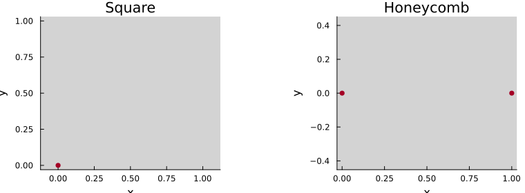

Superlattices and custom filtering

lat_super = Structure.Lattices.superlattice(lat, [[5, -5] [5, 5]])
Structure.Lattices.foldPC!(lat_super)
plot(lat_super, "sublattice"; repeat=[0:2, 0:2], size=(380, 280))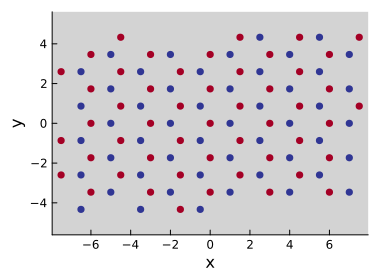

import LinearAlgebra: norm
function honeycomb_holes(; N=12, radius=0.27)
    base = Geometries.honeycomb()
    Structure.Lattices.translate!(base, [1/3, 1/3, 0])
    expanded = Structure.Lattices.superlattice(base, [[N, 0] [0, N]])
    Structure.Lattices.foldPC!(expanded)
    keep = map(x -> norm(x) > radius * norm(Structure.Lattices.getA(expanded)[:, 1]), eachcol(Structure.Lattices.positions(expanded)))
    idx = findall(keep)
    expanded.spacecoordinates = expanded.spacecoordinates[:, idx]
    expanded.extracoordinates = expanded.extracoordinates[:, idx]
    expanded
end
lat_holes = honeycomb_holes(N=12, radius=0.27)
plot(lat_holes, "sublattice"; markersize=2, repeat=[0:2, 0:2], size=(380, 280))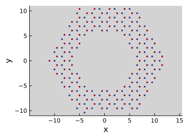

Ribbon reductions

lat_arm = Structure.Lattices.reduceto1D(Geometries.honeycomb(), [[1, 1] [12, -12]])
plot(lat_arm, "sublattice"; supercell=[48], markersize=2, size=(420, 280))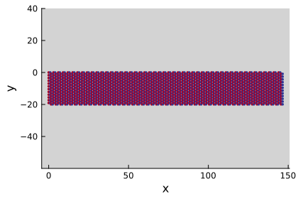

Validation checklist

• Do generated plots match the expected symmetry (e.g. honeycomb sublattices)?
• Are neighbour counts stable when you tweak the cutoff?
• After saving figures, confirm they appear in extra/tutorial/output/.

Suggested extensions

• Swap in Geometries.triangular() or Geometries.square() to compare coordination.
• Attach custom metadata (e.g. layer labels) via the extra_dimensions keyword.
• Feed lattices directly into Operators.graphene and continue with Tutorial 2.