Tutorial 5 — Hofstadter Butterfly

Notebook: extra/tutorial/Tutorial5_Hofstadter.ipynb

Study electrons on lattices subjected to uniform magnetic flux and observe the fractal Hofstadter spectrum.

Learning goals

• Thread magnetic flux through lattice models via Peierls phases or flux attachment helpers.
• Sample dense momentum grids needed to resolve butterfly structures.
• Generate high-resolution spectral plots and density-of-states traces.
• Explore parameter sweeps (flux, onsite energies) to map fine structure.

Prerequisites

• Tutorials 1–2 (lattice construction and band plotting).
• Patience for longer runs—dense k-meshes can take minutes to hours depending on resolution.

Workflow outline

1. Flux insertion — Employ helper routines to add phase factors to hopping terms (see Operators utilities within the notebook).
2. Sampling strategy — Choose grid sizes (klin, kperp, etc.) and tolerances; consider batching to avoid memory spikes.
3. Spectrum calculation — Use Spectrum.getbands or custom sparse solvers to compute eigenvalues across flux values.
4. Visualisation — Plot energy vs. flux butterflies, optionally overlaying integrated density-of-states or gap labelling.
5. Data export — Store arrays for later inspection; the notebook saves .h5/.jld2 files for in-depth analysis.

Live example

figdir = joinpath(pwd(), "figures")
mkpath(figdir)
nothing

ϕs, dos = Operators.hofstadter_dos(
    hops,
    lat,
    16,
    collect(energies);
    klin=36,
    Γ=0.04
)
println("Density of states grid size = ", size(dos))
nothing

Iterating through flux...   3%|▋                        |  ETA: 0:02:10
Iterating through flux...  28%|███████                  |  ETA: 0:00:14
Iterating through flux... 100%|█████████████████████████| Time: 0:00:07
Density of states grid size = (120, 79)

p = heatmap(
    ϕs,
    energies,
    dos;
    xlabel="Flux (ϕ/ϕ₀)",
    ylabel="Energy / t",
    colorbar_title="DOS",
    size=(380, 300)
)
savefig(p, joinpath(figdir, "hofstadter_dos.svg"))
nothing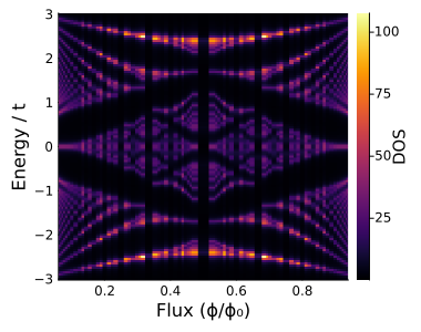

Γ-point spectrum versus flux

flux_list, energies = Operators.hofstadter(hops, lat, 16)
p = scatter(
    [float(ϕ) for (ϕ, e) in zip(flux_list, energies) for _ in e],
    [e for es in energies for e in es];
    ms=1.5,
    alpha=0.6,
    xlabel="Flux (ϕ/ϕ₀)",
    ylabel="Energy / t",
    size=(380, 300)
)
savefig(p, joinpath(figdir, "hofstadter_gamma.svg"))
nothing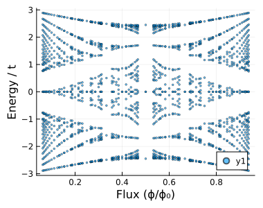

Validation checklist

• Confirm the butterfly reproduces standard graphene features at rational flux values.
• Check that saved data sizes line up with grid dimensions.
• Compare with reference plots in literature for sanity.

Suggested extensions

• Cross-link results with linear-response calculations for quantised Hall conductance.
• Introduce disorder or interaction effects using Meanfield or Superconductivity.
• Automate meshes via extra/examples/graphene/hofstadter.jl for scripted runs.